The experience of being a sports fan can be one of excitement, joy, anxiety, pain, and sometimes all those emotions at the same time. It can create friendships, connect you to a community, and raise your heart rate enough to consider it a form of cardio. When you follow closely enough, you gain an understanding of the sport itself. This understanding of the sport might give rise to an intuition of who will win and even how it could play out, like how many points will be scored in a basketball game. Your intuition gets better the more time you spend watching as you learn more of the nuances. The amazing thing about sports that keeps people watching is, no matter what the person with the most intuition and knowledge of the game thinks, no outcome is guaranteed. There isn't a better example in the world of sports than the NCAA's College Basketball Tournament. Its parody and wild outcomes have earned it the title of March Madness.

The Problem

If you fill out a bracket in March, you know how hard it is to pick a perfect bracket. We still have yet to have a verified perfect bracket in the event's history, which actually isn't surprising given the odds are 1 in 9,223,372,036,854,775,808. It's no one's fault given the exceptional outcomes like Jim Valvano's North Carolina State team winning the National Championship in 1983, the 16 seed UMBC's upset of the overall #1 seed, and every buzzer-beater that seems to freeze time while it is in the air. Let's walk through how you might approach this insurmountable problem of picking your bracket. Along the way, I want to show you that you might know more about machine learning than you think.

Our Approach: Survive and Advance

When we take your first look at the bracket after it is released, we have 63 games to pick (excluding the play-in games). So instead of thinking about the bracket as a whole, let's break it down into a smaller problem: pick the winner of a single game. If we can come up with a consistent rule to pick the winner of a game, then we just have to use that rule 63 times! So let's think of some basic rules and how well they would do. For these rules, let us say each game is between Team A and Team B.

Rule Idea #1: Flip a coin

This is the easiest rule in the book we can use! Fair. Unbiased. So how do we use it? Let's go ahead and define the rule as:

• If the coin lands on heads, then Team A wins
• Otherwise, when the coin lands on tails, Team B wins

So what's the machine learning used here?

The goal of rule #1 is to decide if the winner is “Team A” or “Team B”. These are the two possible outcomes of the game. Another word we can use instead of outcomes here is classes. When we flip the coin, we put the game into one of the two classes: “Team A Win” or “Team B Win”. In machine learning, this is called classification. So in our case here, the coin is our “machine learning classifier”. It is “predicting” which “class” the winner is: “Team A” or “Team B”.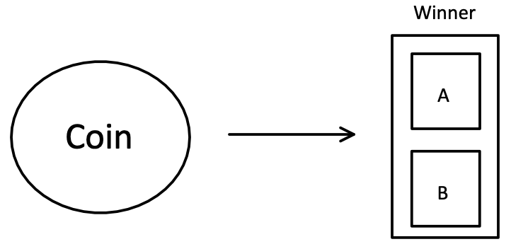(Note: we aren't making predictions here, this is just a function)

Applying Rule #1

We have a 50% chance of predicting the correct winner of an individual game. Not really much to look into here.

Rule Idea #2: The winner is whichever team has the better seed

This is a pretty straightforward idea that performs decently well historically! This rule is extremely biased, which is the purpose of using it. The bias we are using comes from the committee seeding the teams. The committee is made up of experts who take time to study and evaluate each team individually, and the seed they assign a team reflects how good they believe the team to be. If we are to trust these experts, we could use this simple rule. This rule is extremely easy to use, but we run into the problem of what to do when we encounter a game between two teams of the same seed, for that, let's just pick a non-biased comparison like the name of the team's mascot.

• If Team A has a lower seed than Team B, then Team A wins
• If Team B has a lower seed than Team A, then Team B wins
• If Team A and Team B have the same seed, choose whichever team's mascot comes first alphabetically

(Note: the way we describe this “classifier” is still just a function that we can write the outcome to)

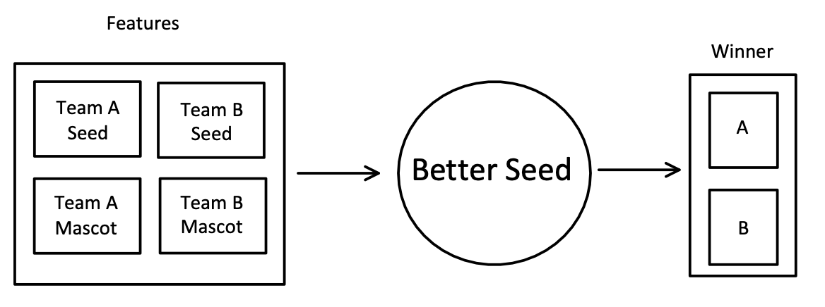
So what's the machine learning used here?

Rule #2 requires us to think about the teams we are comparing. We need two pieces of information about each team: their seed and their mascot. Each piece of information is called a feature in machine learning. Previously, in rule #1, our “classifier” didn't need any information to “predict” which “class” the game fell into. Now, we are going to use two features for each team to “predict” which class the winner is: “Team A” or “Team B”.

Applying Rule #2

Since we have a function we know the outcome to here, we can take a look at last year's tournament to see how well it would have done in 2021. Let's start by taking a peek at results from the East Region.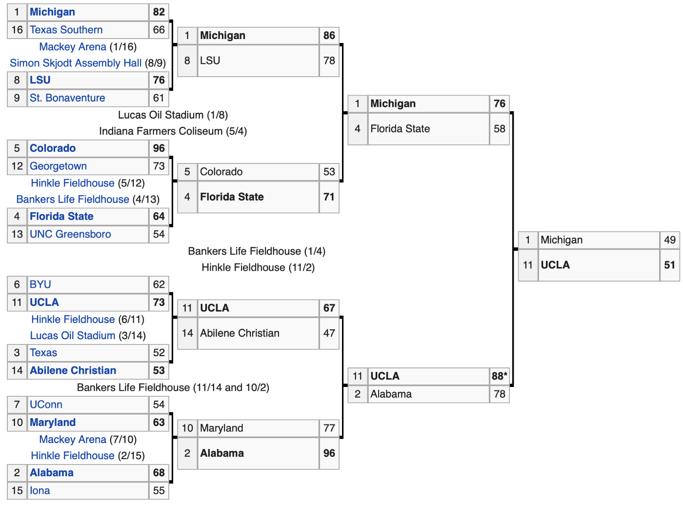Looking at the top half of the regional I am feeling really good about this rule and then…what happened? Well, between an 11 seeded UCLA Bruin team making an incredible run to the Final Four and a 59% free throw shooter hitting two free throws with 1.2 seconds left to beat Texas: we got March Madness'd.
However, looking at the tournament as a whole, we got 66.7% of games correctly classified with our rule! That is looking back at each game individually. If we had been picking from an empty bracket, like we'll be doing this year, we would have only picked 50.8% of the games correctly. So we've got to get smarter about this if we're going to beat our friends this year.

Rule Idea #3: Team Stats

The introduction of information (aka features) gave us a better compass to follow in Rule #2. Right now, we use a small amount of information which allows us to have an easier rule to determine the winner. What if using more information, requiring a more complex rule, gives us better results? Luckily, concerning college basketball, there is a seemingly endless amount of data about teams: strength of schedule, points per game, points allowed per game, free throw percentage, 3pt shooting percentage, etc. Those could be thought of as useful pieces of information. Let's just try using our previous two features with a couple of these new ones. What does our new “classifier” look like?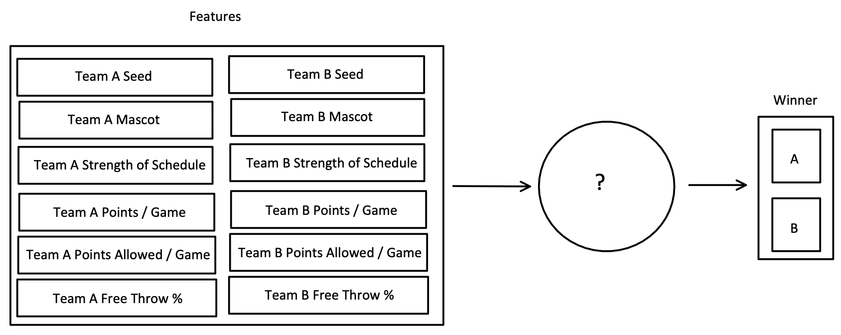Well, we've got our inputs, but think of how many ways we can write a rule to decide the winner. Let's recall how we approached this in Rule #2, we started at the top of our set of information and worked our way down:

1. Compare team seeds
2. If tied, then compare the alphabetical ordering of the team mascots

If we think about what we are doing in our mind here in step 1, we are thinking about the team as a function. We are comparing the value of the two teams. Instead of “Compare team seeds”, let's think about it as “Compare team values”. It just happens that we saying the value of a team is its seed. If we could bust out our 8th-grade math books and write a function to say this, it would be:

Value(team) = seed
I know this would seem to be the opposite of what I am saying since a lower seed means a better team, but for now, think of seed as 17 - seed (e.g. a 1 seed would have a value of 16 and a 16 seed would have a value of 1). So to make use of this new information, we could end up with something like:
Value(team) = seed + (Strength of Schedule) + (Points / Game) - (Points Allowed / Game) + (Free Throw %)
Great! Using more information, we have to be doing better…right? To figure out, we'd go back to evaluating how we did against the last tournament as we did in rule #2. With this new value for the team, maybe we catch some insight we might have missed, like if UCLA played a tougher schedule which helped them get ready for a high-pressure game.

Applying and Improving Rule #3 by Example

Now that we have a more complex rule, let's think about how we will build it piece by piece for the East Regional above.
Say we know that the strength of the schedule will help us correctly pick the winner of UCLA vs BYU, so we add it first to our team value function.
Value(team) = seed + Strength of Schedule
Unfortunately, we forgot that Georgetown's strength of schedule is really high and it incorrectly picks them to beat Colorado. So for those two games, our old seed rule has the same score of 50%. Instead of throwing that stat in the trash can, let's think of another way to allow this information in without it ruining our other prediction. If we just divide the strength of schedule by two, it allows us to still factor that statistic in and we pick both games correctly.
Value(team) = seed + (1/2)*Strength of Schedule
Looking at the rest of that East Region with this rule, we don't miss any other games accidentally. Since we are predicting 1 more correct winner with this rule across this region, let's improve upon it. But let's not just improve upon it, let's get greedy. We know Abilene Christian had the #1 Team Defense Efficiency according to TeamRankings.com, so let's use that to our advantage to predict the coveted 3 vs 14 upset over Texas. Since we only have points allowed per game as a feature, let's multiply it by -1 to give a higher value to teams that allow fewer points per game.
Value(team) = seed + (1/2) * Strength of Schedule + (-1) * Points Allowed / Game
This new team value function gave us what we wanted: predicting Abilene Christian to upset Texas. However, we lost predictions on others that we had previously picked correctly. Now we have to go through all the games again and adjust our team value function to account for them. How we are going to make these adjustments is by just changing the numbers we multiply each statistic by. For example, we changed Strength of Schedule's number from 1 to (1/2). After way more math than any of us wanted to do, we did it.
Value(team) = (0.8)*seed + (0.4)* Strength of Schedule + (-0.5)* Points Allowed / Game
You can see that getting this upset correct while also predicting the other winners took some changes to how we use all the statistics. As long as we have more statistics at our disposal, the resolve to do enough math, and time to run the numbers, we could hopefully reach some rule that predicts the entirety of the East Region correctly. We could even take a step back past that and try to build this team value function that predicts the entirety of last year's tournament correctly.

So what's the machine learning used here?

Rule #3 took some massive steps into the world of machine learning, some of which are too complex to even mention here. The most basic and most important step we took was thinking about our problem through the lens of math. The fundamental idea of using a function to define the value of a team is foundational to machine learning. As we were selecting the statistics that we wanted to use in our team value function, we were going through the practice of what is called feature engineering. The numeric value that we put in front of different statistics (aka features) are called weights in machine learning. Finding the best weights to maximize the number of correct predictions is the process of training (aka fitting) our model. Creating a value for each team and comparing those values to determine the winner of the game allowed us to quantify if we were getting better or worse at predicting. In machine learning, the loss function is this terminology for determining how close you were to the expected predictions.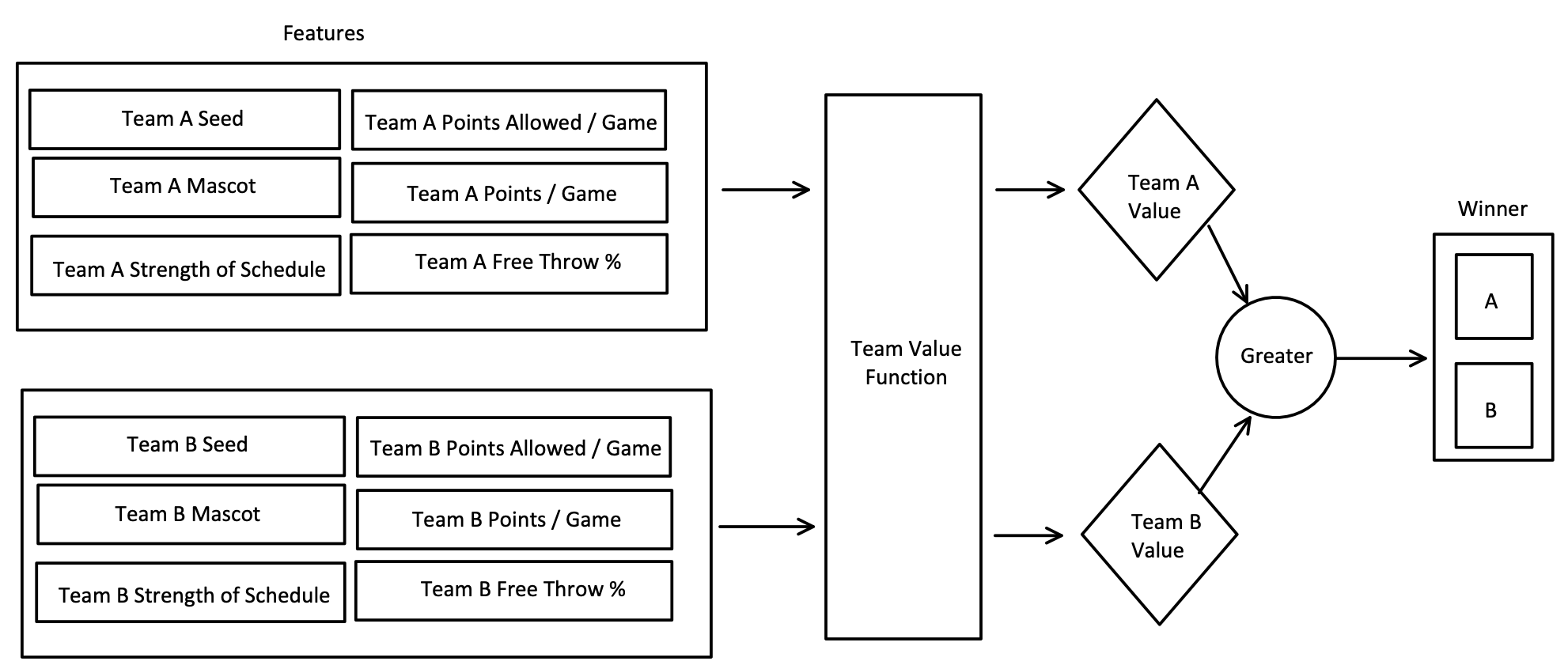

The Bigger Picture

Looking back at our rule #3, we could take as much time adding more stats and adjusting weights to get the rule picking 100% of last year's tournament game winners correctly. The problem is: when you kick back and look proudly upon your work, would you really be confident picking the 15 seeded Oral Roberts to beat the 2 seed Ohio State when the bracket comes out this year? It's okay to be confident if you are because it happened, but you might end up distraught when this year that rule instead picks the upset over a team like the 2 seeded Villanova in 2016 who went on to win the National Championship. This is just to say, defining a one size fits all rule is difficult.
Having built ML models for the last two March Madness tournaments, you gain an even deeper appreciation for the upsets, buzzer-beaters, and each shining moment. In 2019, my model beat me to finish in 1st place in my friend group's pool and in the top 81% of ESPN brackets. In 2021, I beat my model by finishing in the top 98% while my model finished in the top 78%.
In part #2, coming out later this week, we are going expand on the rule #3 classifier through visualizations and dive into actually building a model like this for the 2022 March Madness Kaggle Competition. Hope to see you there!